Why do multi-fact relationships do that?

Part 2 of 2 - Multiple base tables

Part 1 of this series explained how Tableau data models with a single base table create joins. This post will explain the differences with multi-fact relationship models, that is, models with more than one base table.

To follow along with this post, you need to create a Date table, with one row for every day of the year 2193. Why 2193? No idea - that is what is in the bookstore data for dates!

Building on the model from the last post, pull Checkouts into a base table position and create a relationship with Book. (I think of Checkouts like audio books, managed by a third party who only sends data aggregated at a monthly level. Since they are audiobooks, edition isn't relevant and hence the direct connection to Book vs Sales which occur by Edition of book.)

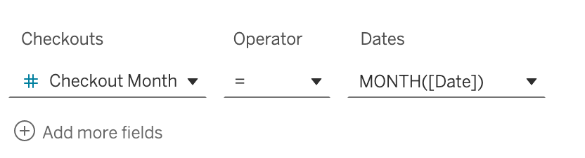
Next step is to create a connection from each of the base tables to the new Date table that was created and brought into the model. Creating a relationship between Sales and Dates is easy, just connect on Sales Date to Date. Checkouts are aggregated to the monthly level. Since there is only one year of data, we can cheat a little and connect on Checkout Month in the Checkouts table to MONTH([Date]) in the dates table:

This is one of the best features of relationships vs joins. We can have tables at different levels of aggregation. One of the other big advantages is that adding new tables to the model doesn't break what we've already built. This would be rare with joins, which almost always break the downstream workbook. And... trying to bring two fact (measure) tables into one big joined table is almost always impossible because there is nothing to join on and the fields don't line up for a union to work.

Next up is the architecture of multi-fact relationships that confuses most people in my experience. What we have now is effectively two different query "trees." If we had 3 base tables, we would have 3 query trees. In other words, one query tree for each base table. And these query trees share downstream tables, which are usually dimension tables in well-architected models. This is why this feature is often called "shared dimensions."

Let's look at how the independent query trees work. When hovering on the right side of a table in the base table position, two arrows pointing together appear.

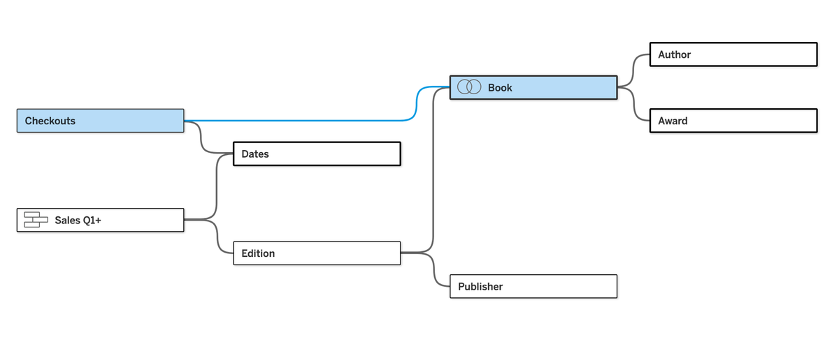
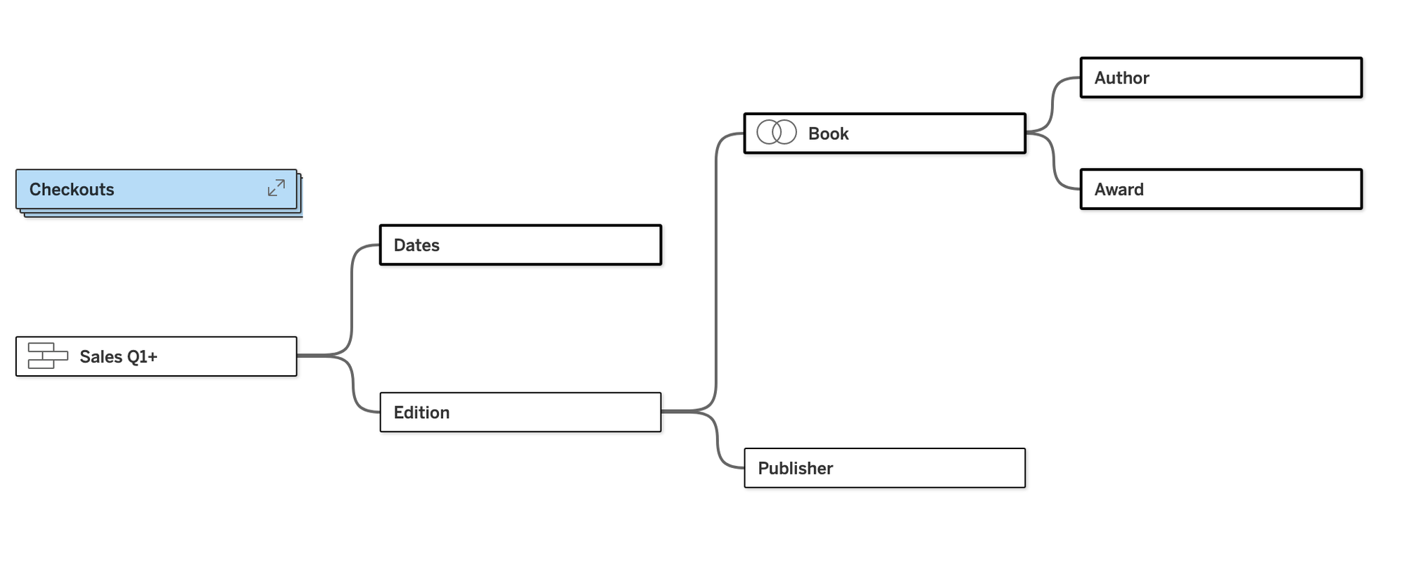
If you click on those arrows, it will collapse the query tree of that base table visually, exposing the other query trees. In this case, closing Checkouts gives us the same model as we had in part 1 of this series (with the exception of the new Date table):

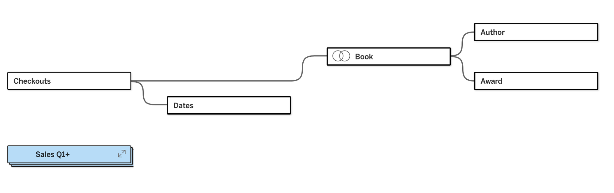
Collapsing the Sales table shows the other tree. Note that Edition and Publisher aren't available as tables to the Checkouts table because they are (literally) unrelated:

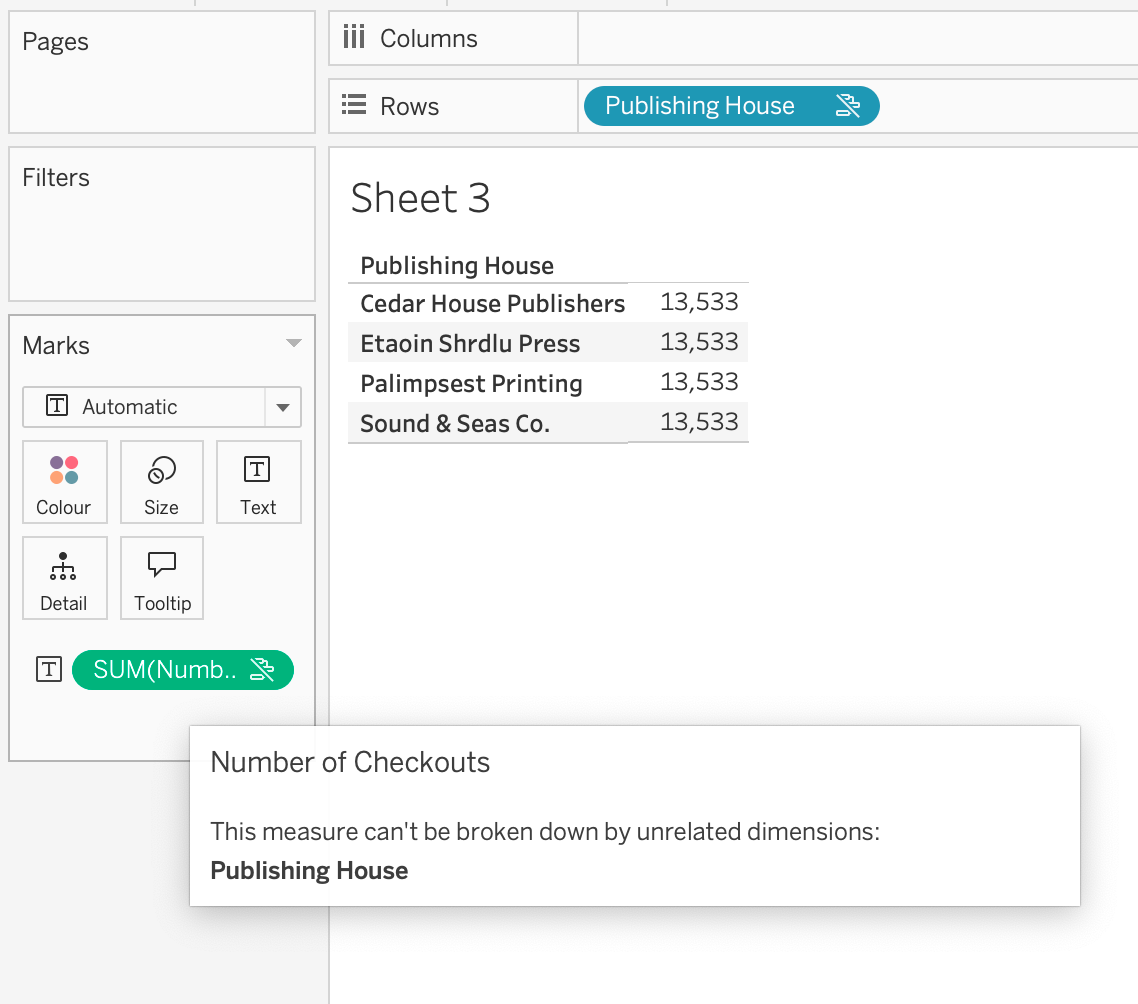
This is part of the reason that it is so important to understand your data model when using relationships, and especially multi-fact relationships. If you want to answer a question like, "what is the breakdown of checkouts by publisher?", you have to know that it isn't possible. Tableau will warn you, but it won't stop you. Pulling in Publishing House, the entire Checkouts table is greyed out in the data pane:

However, it doesn't fully stop you from pulling on a field from that table. The number won't really make sense. It will be all Number of Checkouts in this case. Again, Tableau points this out in a tooltip and makes it clear, but it doesn't stop you:

Ok, let's get back to answers that these multi-fact models can answer. I'm curious about how books are checked out vs sold by genre over time. This is not an answer that is possible in a single query normally. And technically, Tableau isn't able to answer this in a single query either. This is where the brilliance of multi-fact relationships come in. First, this is a very easy question to answer with the model:

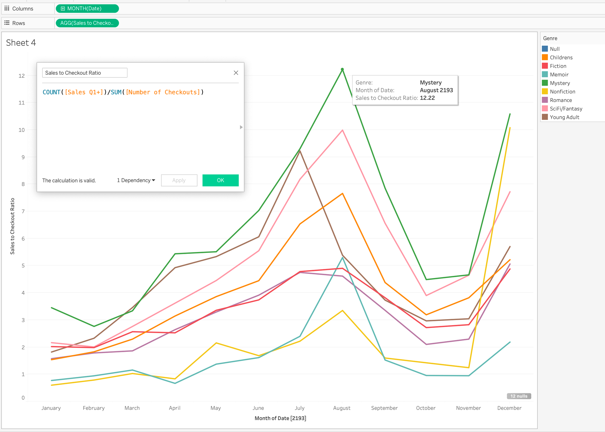
One quick calculation and dragging of three fields and I have my answer. What is Tableau doing? Tableau is issuing two queries. One query is to COUNT the rows in the Sales table (# of Sales) and group it by month and genre. The second query sums the number of checkouts and groups it by month and genre. Then, at the worksheet level, Tableau stitches those queries together to give this correlation visually.

The bookstore use case is a simple one, but think of all the possibilities. And it is these correlations in business that drive the most insight and opportunity to drive real change:
- do sales drop when call goes up?
- does our productivity drop when attrition increases?
- are our sales teams gaming quota by getting customers to buy and then return product?
- how do our customers buy from us across channels?

These are the kinds of questions that used to take time to answer, and usually by data science teams. Now we can get these answers as quickly as any other drag and drop in Tableau.

Before closing out this post, it is important to look at what can't be done with these models and why. The thing that can't be done is row-level calculations across base tables. It makes sense, the only thing that connects them are shared (dimension) tables.

Image a table with sales and another with returns. We can't write a calculation of [Sales $]/[Return $] because how would Tableau know which row(s) to use in the calculation as the tables are only related by shared (dimension) tables. We could write SUM([Sales $])/SUM([Return $]} because Tableau can generate that SQL and return the result without considering which rows in the base tables to use. It can still break down are aggregate calculation by an dimensions we bring into the view.

Looking at this in our dataset requires us first to create a calculation to get Sales Price (it is odd that it doesn't exist in the table already!):

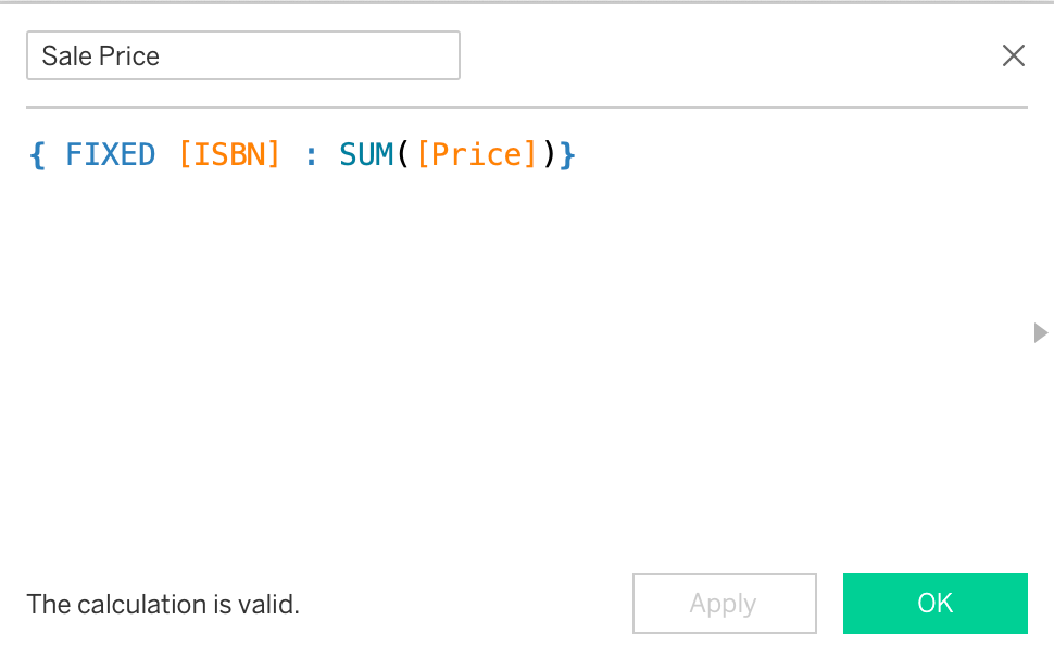
We need to use an LOD only because of the way the data is structured with the price being in the Edition table and not captured in the Sales table itself. (We should also subtract the discount, but I'm going to keep it simple for now).

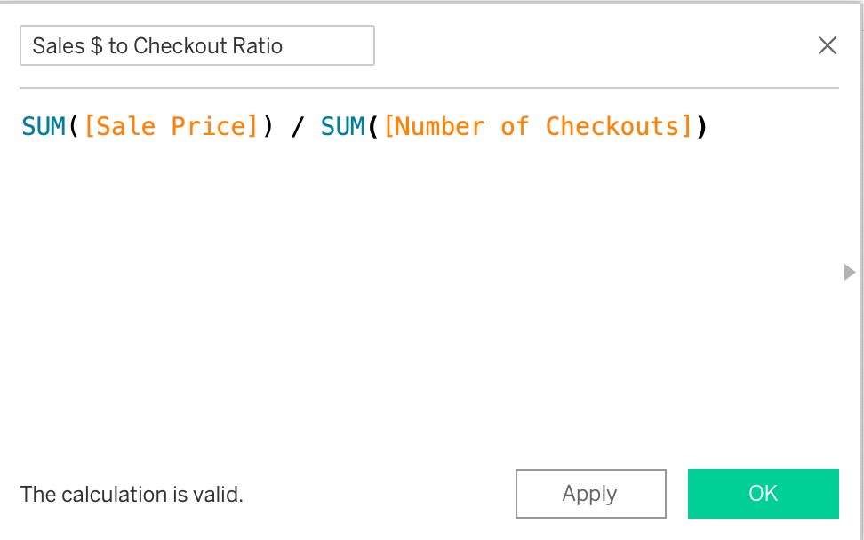
To get how the dollar value of books we sold to checkouts, instead of the volume ratio above, this calculation might come to mind, but won't work:

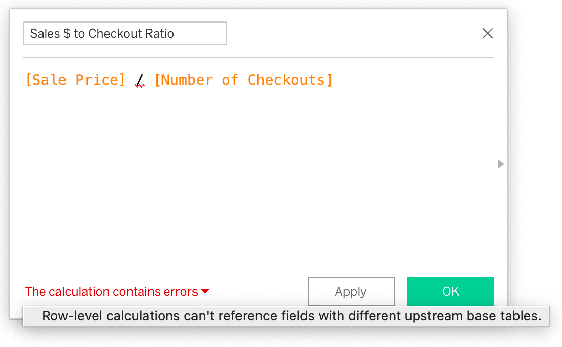
This calculation, which is the right logic anyway, works perfectly fine:

This might seem intuitive to the point where one might ask why I brought it up. Where this catches people is on a certain type of LOD. Let's say I want to break down checkouts by month based on the date a book was first purchased (it doesn't make a lot of sense in this dataset - hang with me).

The following calculation might first seem like an aggregate calculation. We have to remember two things about LODs - they are not materialized (pre-calculated) and although they always have an aggregation in them, they are stored at the row-level.

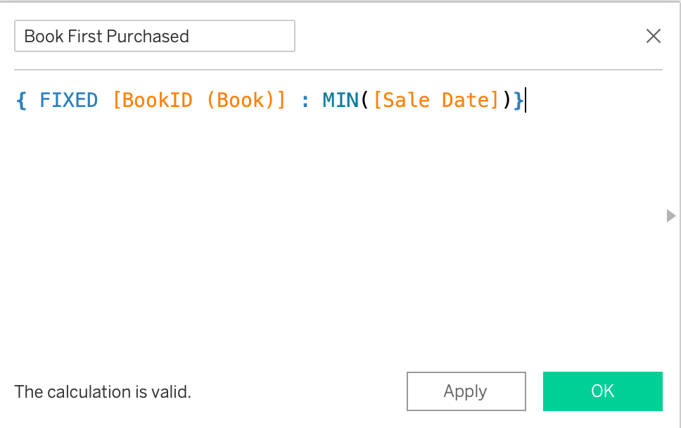
It is intuitive to me that if bring that into a view with checkouts, I could breakdown checkouts by the month the book was first purchased. The reason this doesn't work is that Tableau only runs the calculation when it is brought into the view. Since Sales Date is from a different base table that Checkout Number, each side of that query is aggregated before they are brought together.

To make it work, the first purchase date would need to be materialized (pre-calculated) in the Books table. Alternatively this is one of many cases that can be solved with composable data sources. That is where we are going next!